Mapping an ArcGIS Parcel dataset as a Mapbox tileset
Before I get begin on how I mapped out several large datasets for SanJuanMaps, I would like to say that there was plenty of inspiration behind my actions. I was especially inspired by Justin Palmer’s - The Age of a City. Where he tastefully mapped out all the building ages of Portland, Oregon. But what sets my county maps apart from various other is that I didn’t just map out buildings, people, or objects. I mapped out several sets of data including: building age, building zoning types, current active well sites, and recent crimes.
Loading the Parcel Map
Depending on your city, state, or county it may be a struggle struggle to get a hold of your local GIS information. But for me, I was able to find my counties GIS information for all buildings (not located on federal and/or local reservation land). It took jumping through a few hoops in order to make the data loadable and usable for processing.
To begin San Juan County currently allows you to download a 240MB zip file, thats supposed to contain all GIS information through out the area. This zip file contains numerous files, but the most important one is a dBase file *.dbf. This database table is linked to several ArcGis index files *.atx, meaning that each database column has a unique atx file (phys_address, ownerName, ect). Now that we have access to the GIS dataset, there are a few ways we can access the data in which in contains. Now let me ask; who wants to pay hundreds of dollars to access a GIS file that’ll we’ll be only using a handful of times? Don’t get me wrong, ArcGIS is one hell of a product and if you plan on working with GIS information often or with large datasets it’s worth it. But since this is a one in a blue moon type thing for me I’ll stick with using QGIS, which is an Open-Source GIS projection application. In order to get the application running there are several components that we’ll require, but in the long run it’s well worth.
Now lets= begin with starting up QGIS and opening up the .dbx file as stated before. Since this is a pretty significant file with a ton of datapoints and components, it will take a few moments for everything to load. Once the parcel project loads, you may be faced with a very intricate map that looks similar to CAD wireframe. Your on the right path, lets slow down for a moment. Now an easy way to think of it, is to consider these map components as vector points similar to using the Pen Tool to build shapes in Adobe Illustrator.
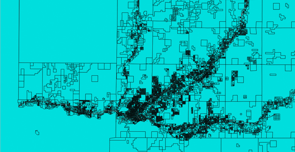
Except this GIS map doesn’t just include points to create a layout of buildings (these is quite a bit of meta-data included with each component on the map). If you zoom in and switch to the Identify Features/vector information tool and click individual plots or buildings you’ll notice it allows you to view information for each parcel. Which consists of tons of information used by the county to identify the area (PARCELNO, GrossAcres, PhysAddr, ACCTTYPE, etc.). Now this doesn’t seem like it’ll be anything important, but when we convert the dBase table to a PostGIS table each one of these attributes will be used as a column to identify each and every building throughout the county.
Understanding Coordinate Reference Systems and Projections
~ Note: This section is not require to read, but helps with understanding why we need to perform a CRS conversion.
Before we get started on converting the parcel dataset to a database table, lets talk about Coordinate Reference Systems (CRS). Wait, why aren’t we just using latitude/longitude? With different maps, we use different coordinate systems. Geographic Coordinate Systems use latitude/longitude and Projected Coordinate Systems use points (X and Y) that originate at a specified lat/long. Think of Projected Coordinate Systems as a window frame, it’s got its one size, area, and dimensions. But no matter how you look at it, all these glass panes end up going together and making one big window.
Lets try to look at why there have been several methods developed to map the Earth’s surface (Mercator, Flamsteed-Sinusoidal, Equal area, Equidistant, Albers, Lambert, and many more). Now I know what your thinking, “What are all these different projections for? And why would I care?” Throughout the years cartographers have experimented with creating projections in which they thought was best for mapping out land, water, cities, and the various features of our planet. And many of them were quite accurate for their time, while others have been slightly narrow minded at depicting the earth.
As we can see, it’s no easy task depicting a spherical planet and all of it’s features as a flat surface. This topographical projection types are called an ellipsoid. No matter what sort of map is used, they have always been an important asset for traveling, freight, military operations, and space travel. Some of these projections are better at depicting land forms, street planning, distances, or scale and accuracy but each one had its place and time. Now the point is, it doesn’t matter if your using degrees (25 is degrees, 35 is minutes, and 22.3 is seconds), meters, decimal degrees (25.58952777777778), or whatever plot point method you should always going to end up at approximately the same place.
So what is a datum? In my opinion the easiest way to explain a datum is by stating it is a standard or method for mapping geographic coordinates to a projection. A datum can consist of various datasets or an individual GIS vector, but generally consists of a large set of data points to be mapped out (roads, buildings, elevation changes, land formations, water, etc).
Mapping with GIS can be a really complicated task, but with the right tools it can make things quite a bit easier.
Let’s convert it to usable data
The ArcGIS data in which we obtained through the county is geo-formatted using the GRS:80 reference system. QGIS will display this and various other attributes when loading up the vector map projection. When looking at the data you should see something similar to the following attributes upon loading up the map.
USER:1000001 (* Generated CRS (+proj=tmerc +lat_0=31 +lon_0=-107.8333333333333 +k=0.9999166666666667 +x_0=829999.9999999998 +y_0=0 +ellps=GRS80 +towgs84=0,0,0,0,0,0,0 +units=us-ft +no_defs))
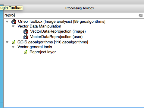
We are now very much on our way to having a data projection of usable data for mapping out the county. The only issue we are going to have at this point is the majority of online mapping tools use the EPSG:4326/WGS84 standard for projecting data. This can easy be achieved by reprojecting the layer with WGS84 coordinates. Go To: Menu -> Processing -> Toolbox -> QGIS geoalgorithms -> Vector General Tools -> Reproject Layer. Another method is if you have the Toolbox side already open you can just search for the tool Reproject Layer
You than set the “Target CRS” as EPSG:4326/WGS84 in the dropdown menu, but we warned depending on your computer this may take a while. Because some of the structures have numerous repetitive points, I had to reduce the point precision in order to keep my computer from freezing up when I would reproject the layer. This can be be found in the toolbox under Grass -> Vector -> v.clean. Be warned if you do need to use this feature, I suggest that you use it sparingly because it can and will readjust the boundaries of various structures.
Now lets save the data as a WTK CSV file, to make it easier to load all the counties properties and their attributes into a database. To do this, rather than saving the project you right-click the Layer and Save-As. From here make sure you need to change the CRS to Default CRS (EPSG:4326 - WGS 84) and that the format is CSV. The next important thing is to force the Geomerty to be expost as AS_WKT and the CSV seperator is COMMA. Now saving may take a while, because there’s quite a few properties that need to have its properties converted to csv.
Many people may not realize it, but CSV files aren’t just large datafiles that you can open up in excel. If you think about, it’s pretty much a plain text database file. It’s a pretty efficient way for accessing data but it can be bulking and slow depending on your editor. With 81000 or so rows, it locks up and freezes Atom and it even slows down Sublime significantly, with 16gb of RAM. But we’re not going to be editing them in an IDE, we’ll be loading them in Postgres. This because Postgres supports GIS data structures and is very efficient at processing large amounts of data.
Before we import the data into Postgres, we need to insure we have proper table structure. And at the moment, one of my favorite tools for building database into out of CSV files by using csvkit. If you’ve never used it, it lets you print column names, convert CSV to JSON, reorder columns, import to SQL, and much more.
Now normally we’d just attempt to build the database scheme with the following command.
csvsql -i postgresql Buildings.csv
But since there are so many rows, the python script will probably freeze up or start consuming a HUGE amount of memory. So in order to make it more efficient, we’ll get the first 20 rows of data. And using command line piping we’ll send the data to the csv tool for processing.
head -n 20 Buildings.csv | csvsql --no-constraints --table buildings
Depending on the information available, your SQL output should be something similar to the following. Several of these columns we’ll never even use, but for now it’s better to not chance corrupting any of our fields. Before you go any farther be sure to change the geometry field names to geom and if CSVKIT labels geom as a VARCHAR for the geometry property type.
CREATE TABLE "buildings" (
  geom geometry,
  ogc_fid INTEGER,
  parcelno BIGINT,
  accountno VARCHAR,
  book INTEGER,
  page INTEGER,
  grossacres FLOAT,
  accttype VARCHAR,
  ownername VARCHAR,
  ownername2 VARCHAR,
  owneraddr VARCHAR,
  ownctystzp VARCHAR,
  subdivis VARCHAR,
  legaldesc VARCHAR,
  legaldesc2 VARCHAR,
  weblink VARCHAR,
  physaddr VARCHAR,
  physcity VARCHAR,
  physzip VARCHAR
);
NOTE: Depending on the GIS software you used, I had various issues with the CSV file that I needed to correct before importing it. The issues that we’ll encounter involve the geometry field. Since CSV fields are separated by commas Postgres tries to import the polygons coordinates as separate columns as well.
POLYGON ((-108.195455993822 36.979941009114)),1,2075189351198,R0051867,,,57.06,EXEMPT,UNITED STATES OF AMERICA US DEPT OF INTE,,6251 COLLEGE BLVD STE A,"FARMINGTON, NM 87402",,A TRACT OF LAND IN THE SESW AND NESW AND NWSE OF 153213 DESCRIBED ON PERM CARD BK.1172 PG.996,,http://propery.url,NM 170,LA_PLATA,
In order to fix this, we need to quote the geometry column in order to make it a field of it’s own. With Sublime’s find/replace REGEX functionality this would be very straight forward step. In order to find the rows with the issue, I used the following ^(?!"POLYGON). Out of 81000 or so columns, there were only a few hundred rows with this issue that needed to be changed.
"POLYGON ((-108.195455993822 36.979941009114,-108.195717330387 36.987213809214,-108.19557299488 36.987214765187))",1,2075189351198,R0051867,,,57.06,EXEMPT,UNITED STATES OF AMERICA US DEPT OF INTE,,6251 COLLEGE BLVD STE A,"FARMINGTON, NM 87402",,A TRACT OF LAND IN THE SESW AND NESW AND NWSE OF 153213 DESCRIBED ON PERM CARD BK.1172 PG.996,,http://propery.url,NM 170,LA_PLATA,
Importing the data into Postgres
Now before we import the dataset, lets enable the PostGIS extension so the database can process the buildings vectors properly.
CREATE EXTENSION postgis;
Now depending on how your managing your database, you either import the CSV file through pgAdmin or through the command line. I chose the the command line, because of its speed and convenience.
copy buildings FROM '/Users/Tarellel/Desktop/SJC_GIS/Exported/Buildings.csv' DELIMITER ',' CSV HEADER;
Compared to loading data in IDE’s and/or Excel, Postgres is extremely fast at accessing, modifying, and deleting rows, columns, and fields. Depending on what data you plan on mapping you may not need to make any additional changes. I’m going to be mapping out all building ages in the county, so I needed to add the built_in column to the table, for the year in which the structure was built.
ALTER TABLE buildings ADD built_in integer;
If you’re like me, you probably already started doing queries to verify the integrity of the information imported. Something you may notice is that the structures geometry field no longer looks like "POLYGON ((-108.195455993822 36.979941009114,-108.195717330387 36.987213809214,-108.19557299488 36.987214765187))". That is because PostGIS stores the locations as a binary specification, but when queried the information is viewed as a hex-encoded string. This makes it easier for PostGIS to store and project the data as various data projection formats.
SELECT geom FROM buildings LIMIT 1;
--------------------
01030000000100000005000000F9A232DD00065BC034E0D442D7594240F0567E50FB055BC094B9B760D55942409E97C29CFE055BC0CAC4E0D8BB594240080B801404065BC0440327CEBD594240F9A232DD00065BC034E0D442D7594240
(1 row)
--------------------
Lets fetch the build/properties initial build date
In order to get each and every buildings initial build date, I ended up using nokogiri to scan the county assessors property listings for their initial build dates. Don’t get me wrong, I tried to look for an easy way to get the information. But they have no publicly accessible API for pulling data requests and never received a response from anyone I attempted to contact. So, I used the next best thing, farmed the counties web site for property listing information.
For warning, This script was build to be quick and simple solution, rather than being well formatted and following best practices.
require 'pg'
require 'open-uri'
require 'nokogiri'
require 'restclient'

# Fetch current buildings across the County and determine their build date
class FetchYear
  @conn = nil
  ###
  # Setup initial required variables, for processing all properties
  # ----------
  # A connection to the database is required for request and updates
  def initialize
    @conn = PG.connect(dbname: 'SJC_Properties')
    @base_link = 'http://county_assessor.url'
  end

  ###
  # Fetches the next X(number) of buildings
  # all selects require that built_in year field to be empty, to prevent an infinite loop
  def fetch_buildings
    @conn.exec('SELECT * FROM buildings WHERE weblink IS NOT NULL AND built_in IS NULL AND built_in != 0 LIMIT 50') do |results|
      # if any results are found, begin processing them to get the properties link/year build
      if results.any?
        results.each do |result|
          # for some reason, some buildings are empty on most fields
          # if no weblink is supplied, skip it
          # ie: "parcelno"=>"2063170454509"
          next if result['weblink'].nil?
          link, built_in = ''
          link = fetch_weblink(result)
          link ||= ''

          # Attempt to fetch the properties build_date
          # Note: some properties are EXEMPT and/or Vacacent
          # so no built_date will be specified
          built_in = (!link.empty? ? fetch_yearbuilt(link) : 0)
          update_build_year(result, built_in)
        end
      else
        puts 'It appears all database rows have been processed'
        abort
      end
    end
  end

  private
  # Private: Fetches the properties unique information URI from the requested
  # SJC assessors page
  # ----------------------------------------
  # building - all attributes for the current building/residence being processed
  # Returns: Returns the properties unique information UIR
  def fetch_weblink(building)
    link = []
    # If it processes successfully attempt to load the Redidental/Commercial page
    # Other output the error
    begin
      # Page required the visitor be logged in as a guest, with a GET form request
      page = Nokogiri::HTML(
                RestClient.get(
                  building['weblink'],
                  cookies: { isLoggedInAsPublic: 'true' }
                )
              )

      # Each property contains a unique URL similar to:
      # http://county_assessor.url/account.jsp?accountNum=R0070358&doc=R0070358.COMMERCIAL1.1456528185534
      # Winthin the left sidebar there is a link table that contains the accttype
      # and based on the accttype/property-type each link will be different
      case(building['accttype'])
      # Select the property when it is a class of Residential
      when 'RESIDENTIAL', 'MULTI_FAMILY', 'RES_MIX'
        link = page.css('#left').xpath('//a[contains(text(), "Residential")]').css('a[href]')

      # Process Commercial based Properties
      when 'COMMERCIAL', 'COMM_MIX', 'MH_ON_PERM', 'PARTIAL_EXEMPT'
        link = page.css('#left').xpath('//a[contains(text(), "Commercial/Ag")]').css('a[href]')

      # Some Vacant and EXEMPT properties only have land listed with no building data available
      # When this is the case or default to no type, return a 0.
      # Because no building info is currently available
      when 'EXEMPT', 'VACANT_LAND', 'AGRICULTURAL'
      else
        return ''
      end

      # Some properties have several links, pull the first/original building info
      first_link(link) if !link.empty?

    rescue OpenURI::HTTPError => e
      if e.message == '404 Not Found'
        puts 'Page not found'
      else
        puts 'Error loading this page'
      end
    end
  end

  def fetch_yearbuilt(link='')
    return '' if link.empty?
    begin
      # Load the URL for the buildings summary
      summary = Nokogiri::HTML(
                  RestClient.get(
                    link,
                    cookies: { isLoggedInAsPublic: 'true' }
                  )
                )
      yearbuilt = summary.css('tr').xpath('//span[contains(text(), "Actual Year Built")]').first.parent.search('span').last.content

      # year must be stripped and turned into an into an integer
      # because it trails with an invisible space ' '
      yearbuilt.strip.to_i
    rescue OpenURI::HTTPError => e
      puts '--------------------'
      puts 'Error loading property summary page'
      puts "URL: #{link}"
      puts '--------------------'
    end
  end

  ###
  # Process the current link:
  # ----------
  # some properties have their attctype listed several times causing errors when processing
  # this is because of upgrades or additions added to the current property
  # Returns the first link for the property array
  def first_link(link)
    link.length <= 1 ? @base_link + link.attribute('href').to_s : @base_link + link[0].attribute('href').to_s
  end

  ###
  # Update the database record with the year it was built
  # ----------
  # record (hash): The current record/addr in which to update
  # year (int): This will be the year/value that needs to be updated in the record
  def update_build_year(record, year='0')
    puts "#{record['accountno']} >/ #{record['physaddr']} - #{year}"
    @conn.exec("UPDATE buildings SET built_in=#{year} WHERE accountno='#{record['accountno']}' AND physaddr='#{record['physaddr']}'")
  end
end

fetch = FetchYear.new
500.times do |x|
  fetch.fetch_buildings
end
I ran this script over night and came back with a fully populated database and ready for to be fully utilized. Depending on the server load, each request usually took a few seconds for each building/property. But one thing that really surprised me, was the counties server had no rate-limiting setup (at least non that I ever experiences). So I was getting results as fast as my script could run and connect. I’m sure the next morning it might of looked like a small DDOS attack by a script kiddy with thousands of page loads from a single source. But I tried to minimize the effect by doing all my data retrieval in the middle of the night, when it would have as little effect as possible.
How the Script Works
Now, before you start scratching your head thinking “what the hell?” let me explain. Each and every property has a unique weblink associated with the count assessors office. When you access the page a cookie isLoggedInAsPublic is set to true, using a get request. I believe this is used in order to prevent general web scraping, because if the cookie isn’t set when the page is loaded redirected to a user login.
I know it looks like a mess and over complicated by let me explain a few things. But some of the properties are owned by the same owner so we can’t exactly relay on the accountno to update properties. And we can’t use physaddr because some properties have more than one building on them, so we rely on updating several properties.
And what about the EXEMPT and Vacant properties? Well the majority of them consists of Churches, Post Offices, Government Buildings, the Airport, and unclassified BLM land. And yes there are quite a few in the generate area. This is the surrounding area is heavily funded by the government, we’re also a city bordering the edge of several reservations.
Lets convert it to a GeoJson file for vectoring
For those of you who have never used used it, Postgres has amazing support for exporting data as json. Some people seem to be unaware that you can resolve to exporting your database queries in different data formats. And some databases (such as Postgres) also allow you to export your database query returns to various file formats.
I can assure you, I didn’t get this right on the first even second try. I’ll honestly admit it took me a few hours to build a query that use the columns I required and would export as a valid GeoJson format. I’d say I probably rebuild the query maybe 20 times, each one being completely different each and everyone. But in the end, I ended up with a swatch of subqueries and assignments that ended exporting the data extremely fast and well structured. As you can see below, the query may look like a complicated mess. The funny thing is, it’s a heck of a lot simpler than some of the other query selections I ended up trying to come up with.
COPY (
  SELECT
    row_to_json(collection)
  FROM(
    SELECT
      'FeatureCollection' AS type,
      array_to_json(array_agg(feature)) AS features
    FROM(
      SELECT
        'Feature' AS type,
        row_to_json(
          (SELECT l FROM
            (SELECT initcap(accttype) AS type, built_in) AS l)
        ) AS properties,
        ST_AsGeoJSON(lg.geom)::json AS geometry
      FROM
        buildings AS lg
      WHERE
        geom IS NOT NULL
      ) AS feature
  ) AS collection
) TO '/Users/Tarellel/Desktop/buildings.json';
Just a heads up you may be expecting a nice and beautiful json structure similar to the following.
Example from geojson-spec data
{ "type": "FeatureCollection",
    "features": [
      { "type": "Feature",
        "geometry": {"type": "Point", "coordinates": [102.0, 0.5]},
        "properties": {"prop0": "value0"}
        },
      { "type": "Feature",
        "geometry": {
          "type": "LineString",
          "coordinates": [
            [102.0, 0.0], [103.0, 1.0], [104.0, 0.0], [105.0, 1.0]
            ]
          },
        "properties": {
          "prop0": "value0",
          "prop1": 0.0
          }
        },
      { "type": "Feature",
         "geometry": {
           "type": "Polygon",
           "coordinates": [
             [ [100.0, 0.0], [101.0, 0.0], [101.0, 1.0],
               [100.0, 1.0], [100.0, 0.0] ]
             ]
         },
         "properties": {
           "prop0": "value0",
           "prop1": {"this": "that"}
           }
         }
       ]
     }
The query I used ends exporting the data more like a crunched dataset. Which is great because it dramatically reduces filesize and is a must when optimizing for loading on webpages. Plus no matter how you use it, it’s not like whatever processor your using is really going to worry about how beautiful your file is, as long as the data is valid.
{"type":"FeatureCollection","features":[{"type":"Feature","geometry":{"type":"Point","coordinates":[102,0.5]},"properties":{"prop0":"value0"}},{"type":"Feature","geometry":{"type":"LineString","coordinates":[[102,0],[103,1],[104,0],[105,1]]},"properties":{"prop0":"value0","prop1":0}},{"type":"Feature","geometry":{"type":"Polygon","coordinates":[[[100,0],[101,0],[101,1],[100,1],[100,0]]]},"properties":{"prop0":"value0","prop1":{"this":"that"}}}]}
Now that you’ve exported the dataset as a GeoJson file, it’s all downhill from here. You’ll just need to use the Mapbox upload API to upload the file. From here you can edit and style the data and vector points the way in which you see fit.
References
- Coordinate Reference Systems
- Overview of Coordinate Reference Systems
- Understanding of Coordinate Reference Systems
- Overview of Coordinate Reference Systems
- Latitude and longitude coordinates are not unique
- Is WGS84 itself a Coordinate Reference System?
- Web-Friendly Geo formats
- Spatial_reference_system
- Geodetic datum
- What’s the difference between a projection and a datum?
- Round Earth, Flat Maps
- GIS : Coordinate Converters
- GeoForms
- Postgres / PostGIS